CNN-Based Single-Image Super-Resolution: A Comparative Study

The following article is a brief report on my Bachelor’s project, a comparative study regarding CNN-Based Single-Image Super-Resolution (SISR) techniques. We’ll begin with a brief look into the first applications of Deep Learning in SISR, followed by a discussion regarding the state-of-the-art CNN-based models for this task. We’ll be comparing the performance of the models on an open-source dataset of satellite images concerning their output quality, speed, and resource demands. You can find the scripts for our experiments as well as the trained super-resolution models here.

Learning in Single-Image Super-Resolution

SISR aims to recover a high-resolution (HR) image from a corresponding low-resolution (LR) version. Given the lower sampling rate of the LR image, smaller details would fall victim to the Nyquist limit, making the problem fundamentally ill-posed, since any combination of amplitudes and phase shifts for the aliased components can yield a valid result for the problem. When you apply a conventional image upsampling technique, such as the bicubic interpolation (BI), to the LR image, the algorithm attempts to fit a specific curve to the 2-d plane of the LR image. It then estimates the HR image pixel values from the interpolated curves.

When the scale factor between the HR image and its LR counterpart surpasses 2, this curve-fitting process results in very smooth images, devoid of sharp edges and sometimes, with “artifacts.” This is because an interpolation technique is not, in fact, adding any new information to the signal. This can be changed with the aid of learning-based techniques. The idea is that if a neural network is provided with enough LR-HR pairs, it will be able to recognize the obscured entities in the LR images and reconstruct them based on the samples it’s seen during training. In other terms, the neural network will learn to “hallucinate” the details lost in the LR image. Deep convolutional neural networks are an obvious candidate for the job, given their outstanding success in image processing problems.

Early Attempts

In their 2014 publication, Chao Dong and his colleagues introduced the first learning-based method for SISR, a deep convolutional neural network that came to be known as SRCNN [1]. Not long after, the same lab published another article, introducing an accelerated version of the same model, unironically called “Fast SRCNN,” or FSRCNN [2], for short, which also improved the performance of the network. FSRCNN makes several modifications to the original SRCNN architecture, enabling it to run in real-time, processing up to 43.5 frames per second with a custom implementation in C++. Real-time processing, unfortunately, has not been a primary goal of the state-of-the-art models. Nevertheless, the structures of these two models have greatly influenced the models that came after. Figure 1 compares the structure of the two. In this figure, Conv(f, n, c) denotes a convolution layer where f, n, and c stand for the filter size, the number of filters, and the number of channels, respectively.

Figure 1. The network structures of SRCNN and FSRCNN. The SRCNN network aims to learn an end-to-end mapping from an upsampled version of the input LR image (using the bicubic algorithm) to the HR target. Instead, FSRCNN introduces a deconvolution layer as the last layer of the network while replacing the non-linear mapping section with a three-step process: shrinking, mapping, and expanding. The authors refer to this as an “hour-glass” structure.

Super-resolution images generated by SRCNN and FSRCNN achieved higher Peak Signal-to-Noise Ratio (PSNR) values than the bicubic interpolation algorithm; e.g., in the famous Set5 dataset, the average PSNR for ×2 super-resolution is increased by around 4dB. Nevertheless, as the scale factor increases, the margin between the two grows smaller. Furthermore, studies have debunked the reliability of the PSNR metric [9] since then, and more recent publications also tend to investigate a more recently-introduced metric known as Structural Similarity (SSIM) [10]. We will be investigating both of these metrics in our study.

Methods

The following models were chosen based on their self-claimed performances on various benchmark datasets. However, there were a couple of models that had reported better results on some of the benchmarks. Still, I was unable to train and/or evaluate them on my setup, and consequently, they were not included in the study. Check out our repository for more details on the implementations. All figures in this section are adapted from their respective works.

Residual Dense Network (RDN)

Residual connections aren’t exactly a new idea in SISR models. Several older studies have also utilized these connections to improve the network's training, such as [11]. However, the authors in [3] take it to the extreme and introduce the Residual Dense Blocks (RDB), illustrated in Figure 2.

Figure 2. Residual Dense Blocks, the main building block of RDN.

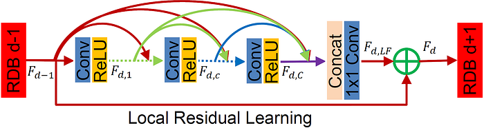
The overall structure of the network is rather simple. The architecture of RDN is rather similar to FSRCNN, in the sense that it begins with convolution layers for feature extraction and ends with an upsampling operator (with learnable parameters) that maps the extracted features to the HR space. The upsampling operator in this network is inspired by [13]. In between the two, D RDB blocks are stacked on top of one another, the outputs of which are then concatenated and passed through a convolution layer with 1×1 filters.

Figure 3. The architecture of RDN.

The authors use the L₁ loss function and the Adam optimizer for training the network. To stabilize the training procedure, the learning rate is decreased exponentially every certain number of epochs. Later works have also adopted this setting. Despite its complicated architecture, RDN is the fastest one to train and is also among the top two with regard to inference time. Besides, RDN is one of the few models that I could train and evaluate on my notebook’s NVIDIA GTX 1660 Ti with only 6GB of VRAM. Yet, RDN is the second largest model with respect to learnable parameter counts, which speaks volumes about its efficiency.

Residual Channel Attention Network (RCAN)

[4] is perhaps the most influential work in this list, spawning several other models based on its architecture, one of which is in this list! The most fundamental innovation of this work is the Channel Attention (CA) mechanism, which the authors claim can extract useful channel-wise features from the inputs.

Figure 4. Channel Attention mechanism introduced in [4].

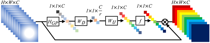
At the start of the CA mechanism, a global average pooling (GP) is applied to the input, transforming it into a 1×1×C tensor, which is then passed through a convolution layer (D), a deconvolution layer (U), and the logistic sigmoid activation function (f).

Figure 5. The structure of RCABs.

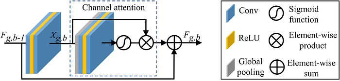
This mechanism is then embedded in Residual Channel Attention Blocks (RCABs; Figure 5), which are the primary building block of RCAN, as illustrated in Figure 6.

Similar to RDN, the upscaling module in RCAN is inspired by the ideas introduced in [13].

Figure 6. The architecture of RCAN.

The computation cost of the attention mechanism in this network significantly increases the model's resource demand, making it one of the hardest ones to work with on this list. Another noteworthy point regarding this model is that RCAN is the only model on this list preferred using the Stochastic Gradient Descent to the Adam optimizer. However, the authors still use learning rate scheduling with similar settings for more stable training.

Super-Resolution Feedback Network (SRFBN)

Before the work of [5], the utilization of feedback mechanisms, which have a biological counterpart in the human visual system, had been explored in various computer vision tasks, but not super-resolution. The authors place a structure, which they refer to as the Feedback Block (FB), with several consecutive pairs of convolution and deconvolution pairs, each proceeded by a 1×1 convolution layer, under a feedback connection. The inner structure of the FB is illustrated in Figure 7. The authors

Figure 7. The structure of FB.

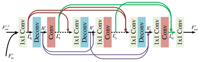
This structure is then put into the architecture illustrated in Figure 8. An important feature of the SRFBN model, apparent from the figure, is that rather than learning an end-to-end mapping from the LR space to the HR space, the convolutional layers are tasked with predicting the residual error between the HR image and a copy of the LR input which has been upsampled by the bicubic interpolation algorithm. This technique, which is referred to as residual learning, has been studied in some previous works (earliest being [14]) and has shown to considerably speed up the model's convergence, reaching satisfactory quality in far fewer epochs than end-to-end models.

Figure 8. The structure of SRFBN (to the left) and unfolded (to the right). Layers labeled as LRFB are the LR Feature extraction Block, and the couple labeled as RB is the Reconstruction Block, which maps the extracted features into an RGB image.

Thanks to the feedback mechanism, the network is able to achieve qualities very close to the other methods but with the least number of learnable parameters. I trained this model on my notebook, but the evaluation script is rather excessive in memory consumption (to avoid disk I/O operations, as far as I understood). Inference through this technique is also rather quick, usually as fast as RDN.

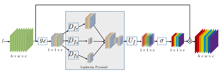
Densely Residual Laplacian Network (DRLN)

The model introduced in [6], is heavily inspired by the RCAN model and is merely attempting to push the boundaries with the RCAN architecture. The authors modify the Channel Attention mechanism and replace the earliest convolution layer in CA with several dilated convolutions, with different dilations. This novel attention mechanism, which they refer to as Laplacian Attention, is shown in Figure 9.

Figure 9. The structure of the Laplacian Attention mechanism. The subscripts in the Laplacian Pyramid denote the dilation factor of the respective convolution layers.

The architecture of this model is illustrated in Figure 10. The architecture is similar to that of RCAN, with short residual connections bypassing several consecutive building blocks and one long connection, connecting the features extracted from the LR image to the groups' final output. However, DRLN applies its attention mechanism less frequently than RCAN and instead adds several convolution layers after its smaller building blocks, which they refer to as Dense Residual Laplacian Modules (DRLMs).

Figure 10. The structure of DRLN. In this figure, residual connections are referred to as skip connections.

The authors certainly achieve their goal of pushing the model to its limits and double the number of learnable parameters while also reducing the time needed for both training and inference. However, this complicated model does not improve the quality of the output images (at least for our dataset) and only performs as well as RCAN.

Gated Multiple Feedback Network (GMFN)

The model introduced in [7] is a follow-up work by the authors of SRFBN, with the aim to introduce multiple hierarchical feedback connections into the model to increase the quality of the SR images. The authors retain the residual learning paradigm and the couple of convolution layers tasked with extracting features from the LR image from SRFBN. However, the FB is entirely replaced by an array of RDBs (introduced in [3] for the RDN model) with dense feedback connections controlled by Gated Feedback Modules (GFMs). GFMs select useful information from high-level features (features extracted in the previous iteration) for further refinements. The structure of the GFMs, as well as the GMFN model, is illustrated in Figure 11.

Figure 11. The structure of GMFN, GFM, RDB (identical to the one introduced in RDNs), and the reconstruction block (identical to the final layers in the SRFBN model).

The authors' changes made push the quality of the SR images generated by GMFN significantly above SRFBN while also reducing the runtime of inference, with a small penalty to the training time. Moreover, the GMFN model manages to surpass the RDN model in quality with fewer RDBs. In our experiments, the margin between the quality of the interpolated images and the SR images reduces more slowly for GMFN compared to other models, hinting that GMFN is the superior technique in higher scale factors.

Cross-Scale Non-Local Network (CSNLN)

Figure 11. Non-local cross-scale similarities in an image.

The authors of [8] call on an older idea used by traditional methods for SISR, self-similarity, which can be excellently described using the example in Figure 11. In this image, several larger patches throughout the image are similar to the target patch we’re trying to upscale. These patches can serve as a guide in reconstructing the target patch in the SR image.

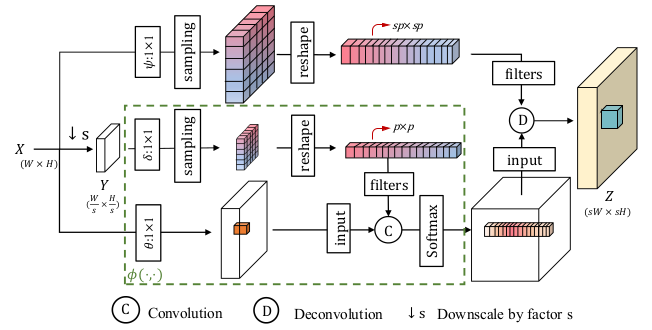
The authors introduce two new attention mechanisms, designed for exploiting self-similarity. In-Scale Non-Local Attention (ISNLA) is a computationally expensive attention mechanism that can expose self-similarities in the image on the same scale. Cross-Scale Non-Local Attention (CSNLA) is the more convoluted sibling of ISNLA, finding similar patches with different sizes. Figure 12 shows the structure of the CSNLA mechanism.

Figure 12. The structure of the CSNLA mechanism. The upper branch looks for the patches in the LR image corresponding to patches in the HR image, while the branches within the green box find the similarities.

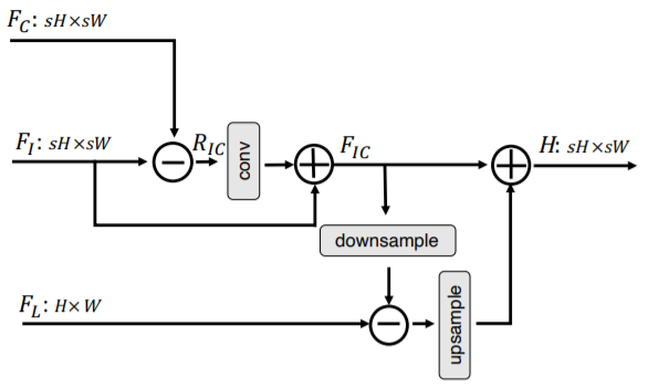
The CSNLN model applies these attention mechanisms to features extracted by convolution layers and then combines them with the features themselves using an approach they refer to as mutual-projected fusion. This procedure is shown in Figure 13.

Figure 13. The mutual-projected fusion. The upsample operation, as well as the downsample operation, are implemented using convolutional layers. The lower input denoted as L is the features extracted by the convolution layers processed by the attention mechanisms. s refers to the scale factor for the SR transformation.

The attention mechanisms and the convolution layers previously discussed are first upscaled via a deconvolution layer, followed by a couple of ReLU-activated convolutional layers. These building blocks form a Self-Exemplars Mining (SEM) cell, illustrated in Figure 14, along with the overall architecture of CSNLN. CSNLN uses feedback connections similar to SRFBN, putting its main building block within one.

Figure 14. The unfolded structure of CSNLN. Features extracted with each iteration are collected and concatenated into the same tensor.

The convoluted attention mechanisms introduced in this work can give it an edge in reconstruction quality in lower scale factors. However, this slight edge comes at an incredible cost, increasing both the training time and inference time of the model by order of magnitude, even though the network itself is a moderate-size network regarding the number of learnable parameters has.

Performance Evaluation and Comparison

We based our experiments on a similar study, [15], to draw a direct comparison between the models discussed above and the older approaches discussed in this article. We use the open-source Draper Satellite Image Dataset, which consists of 1720 RGB images, all 3099×2329 pixels. The first 350 images in this dataset are used as the train set, while the remaining 1370 are center-cropped to 720×720 and used as the test set.

All models were trained and tested with the hyperparameters and optimization settings suggested in their source code repositories on an NVIDIA V100 Volta with 32GB of VRAM. Note that the implementations are in various versions of PyTorch and use different versions of the CUDA library, which might have a small effect on their speed. The reported inference times are the average values recorded when reconstructing the entire dataset. We use the implementation of the bicubic interpolation algorithm provided in the Scikit-Image library, which might not be the most efficient implementation. Still, the same can be said for the CNN-based models.

Table 1 shows the results of our experiments.

Table 1. Comparison of the CNN-Based Single-Image Super-Resolution techniques, regarding reconstruction quality, no. of learnable parameters, training time, and inference time. The best value for each metric has been bolded. VDSR, SRGAN, and EEGAN are not discussed in this article. Refer to [14], [16], and [15], respectively.

To summarize, it seems that the idea of feedback networks can greatly help out SISR models; these networks can keep up with models with far more learnable parameters and deliver the same quality of reconstruction. Furthermore, it seems that while attention mechanisms seem to be the superior technique with small scale factors, where we want to recover minor details, techniques without one often surpass these techniques in higher scale factors, rendering their computational cost unreasonable to bear. If you’d ask us, we’d go with RDN or GMFN, depending on whether we can endure a little longer training for faster inference.

[1] Dong, Chao, Chen Change Loy, Kaiming He, and Xiaoou Tang. “Image super-resolution using deep convolutional networks.” IEEE transactions on pattern analysis and machine intelligence 38, no. 2 (2015): 295–307.

[2] Dong, Chao, Chen Change Loy, and Xiaoou Tang. “Accelerating the super-resolution convolutional neural network.” In European conference on computer vision, pp. 391–407. Springer, Cham, 2016.

[3] Zhang, Yulun, Yapeng Tian, Yu Kong, Bineng Zhong, and Yun Fu. “Residual dense network for image super-resolution.” In Proceedings of the IEEE conference on computer vision and pattern recognition, pp. 2472–2481. 2018.

[4] Zhang, Yulun, Kunpeng Li, Kai Li, Lichen Wang, Bineng Zhong, and Yun Fu. “Image super-resolution using very deep residual channel attention networks.” In Proceedings of the European Conference on Computer Vision (ECCV), pp. 286–301. 2018.

[5] Li, Zhen, Jinglei Yang, Zheng Liu, Xiaomin Yang, Gwanggil Jeon, and Wei Wu. “Feedback network for image super-resolution.” In Proceedings of the IEEE Conference on Computer Vision and Pattern Recognition, pp. 3867–3876. 2019.

[6] Anwar, Saeed, and Nick Barnes. “Densely residual laplacian super-resolution.” IEEE Transactions on Pattern Analysis and Machine Intelligence (2020).

[7] Li, Qilei, Zhen Li, Lu Lu, Gwanggil Jeon, Kai Liu, and Xiaomin Yang. “Gated multiple feedback network for image super-resolution.” arXiv preprint arXiv:1907.04253 (2019).

[8] Mei, Yiqun, Yuchen Fan, Yuqian Zhou, Lichao Huang, Thomas S. Huang, and Honghui Shi. “Image super-resolution with cross-scale non-local attention and exhaustive self-exemplars mining.” In Proceedings of the IEEE/CVF Conference on Computer Vision and Pattern Recognition, pp. 5690–5699. 2020.

[9] Wang, Zhou, and Alan C. Bovik. “Mean squared error: Love it or leave it? A new look at signal fidelity measures.” IEEE signal processing magazine 26, no. 1 (2009): 98–117.

[10] Wang, Zhou, Alan C. Bovik, Hamid R. Sheikh, and Eero P. Simoncelli. “Image quality assessment: from error visibility to structural similarity.” IEEE transactions on image processing 13, no. 4 (2004): 600–612.

[11] Lim, Bee, Sanghyun Son, Heewon Kim, Seungjun Nah, and Kyoung Mu Lee. “Enhanced deep residual networks for single image super-resolution.” In Proceedings of the IEEE conference on computer vision and pattern recognition workshops, pp. 136–144. 2017.

[13] Shi, Wenzhe, Jose Caballero, Ferenc Huszár, Johannes Totz, Andrew P. Aitken, Rob Bishop, Daniel Rueckert, and Zehan Wang. “Real-time single image and video super-resolution using an efficient sub-pixel convolutional neural network.” In Proceedings of the IEEE conference on computer vision and pattern recognition, pp. 1874–1883. 2016.

[14] Kim, Jiwon, Jung Kwon Lee, and Kyoung Mu Lee. “Accurate image super-resolution using very deep convolutional networks.” In Proceedings of the IEEE conference on computer vision and pattern recognition, pp. 1646–1654. 2016.

[15] Jiang, Kui, Zhongyuan Wang, Peng Yi, Guangcheng Wang, Tao Lu, and Junjun Jiang. “Edge-enhanced GAN for remote sensing image superresolution.” IEEE Transactions on Geoscience and Remote Sensing 57, no. 8 (2019): 5799–5812.

[16] Ledig, Christian, Lucas Theis, Ferenc Huszár, Jose Caballero, Andrew Cunningham, Alejandro Acosta, Andrew Aitken et al. “Photo-realistic single image super-resolution using a generative adversarial network.” In Proceedings of the IEEE conference on computer vision and pattern recognition, pp. 4681–4690. 2017.